Spotify Hits
It doesn’t take an avid music listener to notice that many popular songs have the same formula to them. Radio stations can often sound like the same song is playing on repeat, with slightly different variants of the same song gaining recognition and winning awards.
This very thought led me to find a Spotify dataset that contained all Billboard top 10 songs from the years 2010 to 2019. All there was left to do was explore it a bit.
I started by doing some exploratory analysis of the dataset. While the categorical variables are self-explanatory, here’s a key for the quantitative variables for reference:
- acousticness (Ranges from 0 to 1)
- danceability (Ranges from 0 to 1)
- energy (Ranges from 0 to 1)
- duration_ms (Integer typically ranging from 200k to 300k)
- instrumentalness (Ranges from 0 to 1)
- valence (Ranges from 0 to 1)
- popularity (Ranges from 0 to 100)
- tempo (Float typically ranging from 50 to 150)
- liveness (Ranges from 0 to 1)
- loudness (Float typically ranging from -60 to 0)
- speechiness (Ranges from 0 to 1)
summary(topten)
##        X            title              artist           top.genre
##  Min.   :  1.0   Length:603         Length:603         Length:603
##  1st Qu.:151.5   Class :character   Class :character   Class :character
##  Median :302.0   Mode  :character   Mode  :character   Mode  :character
##  Mean   :302.0
##  3rd Qu.:452.5
##  Max.   :603.0
##       year           bpm             nrgy           dnce
##  Min.   :2010   Min.   :  0.0   Min.   : 0.0   Min.   : 0.00
##  1st Qu.:2013   1st Qu.:100.0   1st Qu.:61.0   1st Qu.:57.00
##  Median :2015   Median :120.0   Median :74.0   Median :66.00
##  Mean   :2015   Mean   :118.5   Mean   :70.5   Mean   :64.38
##  3rd Qu.:2017   3rd Qu.:129.0   3rd Qu.:82.0   3rd Qu.:73.00
##  Max.   :2019   Max.   :206.0   Max.   :98.0   Max.   :97.00
##        dB               live            val             dur
##  Min.   :-60.000   Min.   : 0.00   Min.   : 0.00   Min.   :134.0
##  1st Qu.: -6.000   1st Qu.: 9.00   1st Qu.:35.00   1st Qu.:202.0
##  Median : -5.000   Median :12.00   Median :52.00   Median :221.0
##  Mean   : -5.579   Mean   :17.77   Mean   :52.23   Mean   :224.7
##  3rd Qu.: -4.000   3rd Qu.:24.00   3rd Qu.:69.00   3rd Qu.:239.5
##  Max.   : -2.000   Max.   :74.00   Max.   :98.00   Max.   :424.0
##      acous            spch             pop
##  Min.   : 0.00   Min.   : 0.000   Min.   : 0.00
##  1st Qu.: 2.00   1st Qu.: 4.000   1st Qu.:60.00
##  Median : 6.00   Median : 5.000   Median :69.00
##  Mean   :14.33   Mean   : 8.358   Mean   :66.52
##  3rd Qu.:17.00   3rd Qu.: 9.000   3rd Qu.:76.00
##  Max.   :99.00   Max.   :48.000   Max.   :99.00
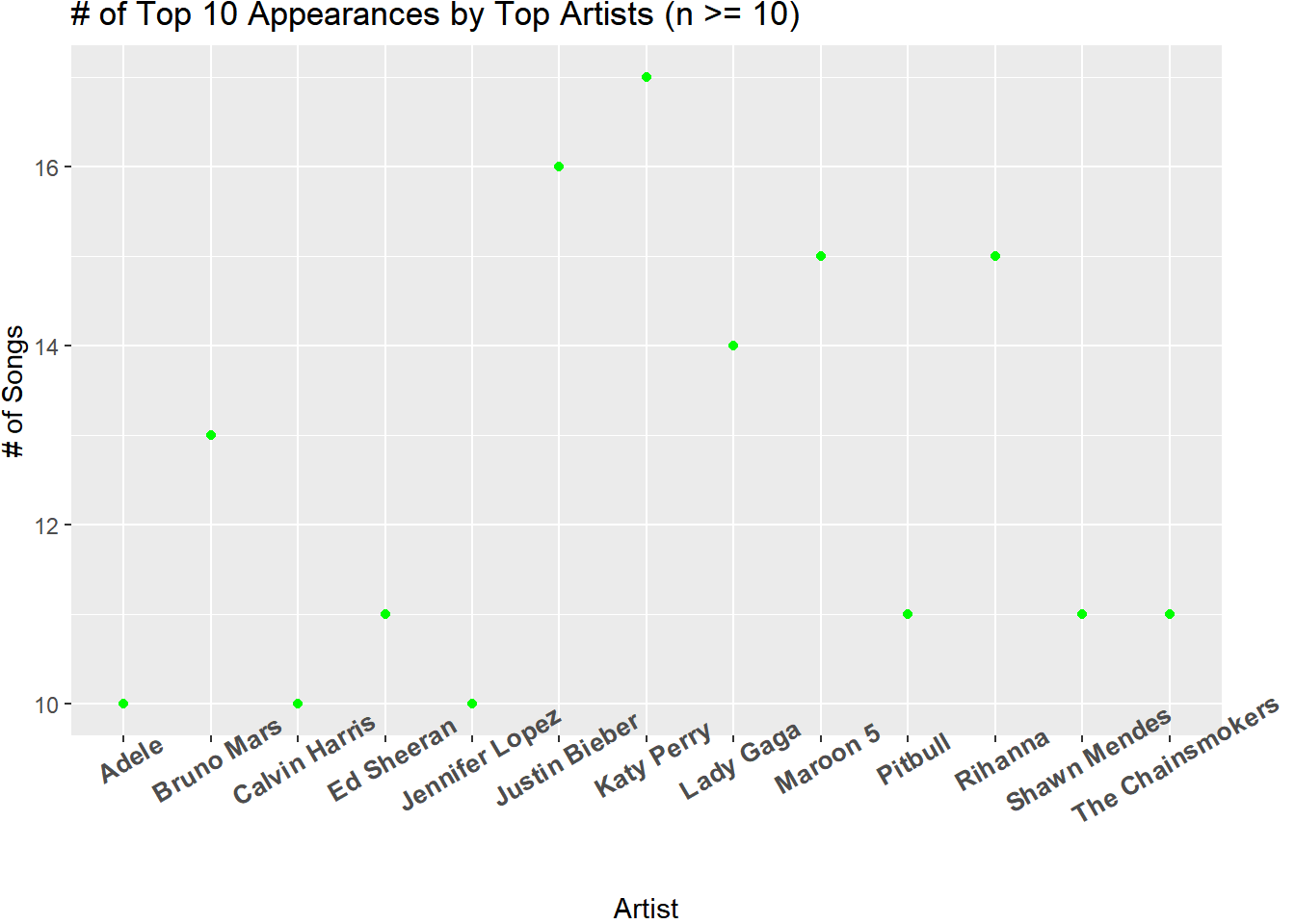
Songs that generally have the same sound could be explained by a number of reasons, such as coming from the same genre or artist. With that in mind, I wanted to explore the relationship between top songs and the artist making them.
| # of Genres for Artists with Multiple Hits | ||
|---|---|---|
| For each artitst with multiple hits in a year, in how many genres were their hits? | ||
| Year | # of Genres | # of Artists |
| 2010 | 1 | 12 |
| 2011 | 1 | 12 |
| 2012 | 1 | 9 |
| 2013 | 1 | 16 |
| 2014 | 1 | 7 |
| 2015 | 1 | 20 |
| 2016 | 1 | 18 |
| 2017 | 1 | 15 |
| 2018 | 1 | 13 |
| 2019 | 1 | 6 |
This brief investigation tells us the top artists over the 10-year period as well as the fact that their respective hits were all within the same genre. This implies that artists are hesitant to change the formulas that bring them success. Or that listeners aren’t interested in the songs that do change that formula.
I then started wondering about one-hit wonders and the effect that the addition of new streaming platforms had on the variety of artists that created hits.
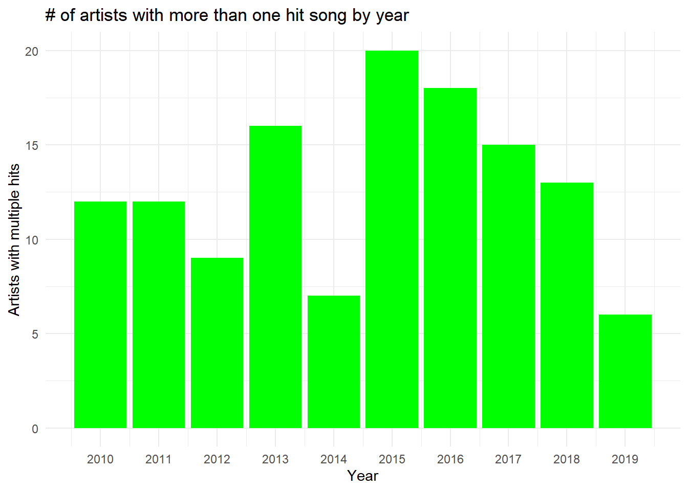 It’s hard to find a trend in the first half of the decade. However, after the spike in 2015, there’s a marked decrease in the number of artists that were able to produce multiple hit songs within a year. Rather than attributing this trend solely to streaming platforms, it may also be a byproduct of increasing ways to produce music.
Me, Myself, and I by G-Eazy was unmistakably one of the biggest hits on the radio when it was released. Though what I found most interesting was the number of songs that went by the same title though created by different artists (Big Sean and Beyonce to name a couple) in different genres. This led me to investigate whether the subject of a song, expressed by its title, had an effect on whether it would be a hit.
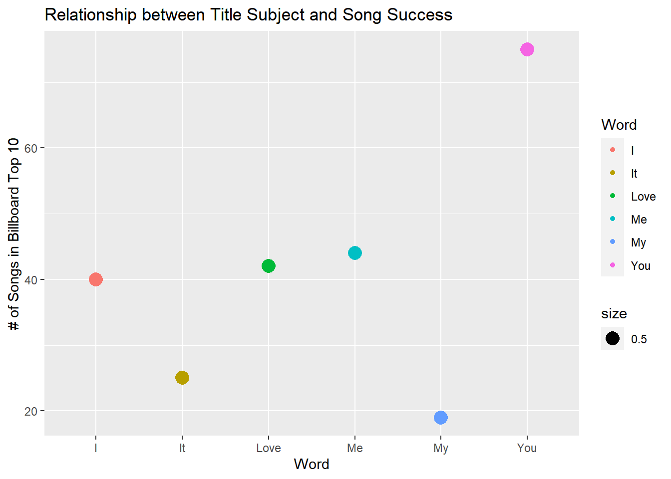
I did realize there is a level of overlap, such as the possibility that a song title has multiple subjects and even a verb, allowing a song titled “I Love You” to be cross-listed 3 times. Despite this, “Love” had particularly interesting results in my opinion. Being the only word that is both a noun and a verb, I expected it to appear more often than all except for “You” which was understandably common.
Finally, I’m sure you’ve noticed the variable “pop” is intuitively related to the likelihood that a song would be in the Billboards Top 10. So I ventured to identify the relationship between the other quantitative variables and a song being a Billboards Number 1. For this, I created a dummy variable that represented whether a song was ever a Billboards Number 1.
Unfortunately the target data is very unbalanced, with only 72 of 603 observations having been a billboards number 1. In an attempt to build a substantive model, I tried both oversampling and undersampling. But before that, I created a model using random forest with the unbalanced data to demonstrate the issue.
## Confusion Matrix and Statistics
##
##           Reference
## Prediction  no yes
##        no  105  13
##        yes   0   2
##
##                Accuracy : 0.8917
##                  95% CI : (0.8219, 0.941)
##     No Information Rate : 0.875
##     P-Value [Acc > NIR] : 0.3502795
##
##                   Kappa : 0.2121
##
##  Mcnemar's Test P-Value : 0.0008741
##
##             Sensitivity : 1.0000
##             Specificity : 0.1333
##          Pos Pred Value : 0.8898
##          Neg Pred Value : 1.0000
##              Prevalence : 0.8750
##          Detection Rate : 0.8750
##    Detection Prevalence : 0.9833
##       Balanced Accuracy : 0.5667
##
##        'Positive' Class : no
##
Based on the “No Information Rate” it’s clear that there’s such a strong majority in the target feature, the model simply predicts that practically no songs are Billboards number 1s. This leads to a good accuracy score but awful kappa and specificity scores.
Think of the kappa value as being indicative of how much of the prediction would be accurate even if all predictions were allocated to the majority class, 1 indicating it’s a useful model despite unbalanced data and 0 meaning it isn’t helpful.
To address this, first I tried undersampling and arrived at the following output.
## Confusion Matrix and Statistics
##
##           Reference
## Prediction no yes
##        no  50   8
##        yes 55   7
##
##                Accuracy : 0.475
##                  95% CI : (0.3831, 0.5682)
##     No Information Rate : 0.875
##     P-Value [Acc > NIR] : 1
##
##                   Kappa : -0.0244
##
##  Mcnemar's Test P-Value : 6.814e-09
##
##             Sensitivity : 0.4762
##             Specificity : 0.4667
##          Pos Pred Value : 0.8621
##          Neg Pred Value : 0.1129
##              Prevalence : 0.8750
##          Detection Rate : 0.4167
##    Detection Prevalence : 0.4833
##       Balanced Accuracy : 0.4714
##
##        'Positive' Class : no
##
While the undersampled model had a more even distribution of predictions for each class, this resulted in a test accuracy score that’s worse than a theoretical coin flip.
The random forest model with oversampling resulted in the following output.
## Confusion Matrix and Statistics
##
##           Reference
## Prediction  no yes
##        no  105  13
##        yes   0   2
##
##                Accuracy : 0.8917
##                  95% CI : (0.8219, 0.941)
##     No Information Rate : 0.875
##     P-Value [Acc > NIR] : 0.3502795
##
##                   Kappa : 0.2121
##
##  Mcnemar's Test P-Value : 0.0008741
##
##             Sensitivity : 1.0000
##             Specificity : 0.1333
##          Pos Pred Value : 0.8898
##          Neg Pred Value : 1.0000
##              Prevalence : 0.8750
##          Detection Rate : 0.8750
##    Detection Prevalence : 0.9833
##       Balanced Accuracy : 0.5667
##
##        'Positive' Class : no
##
The oversampled model ended up creating the same predictions as the original model, which again is a good accuracy score, but doesn’t mean that the model is necessarily useful.
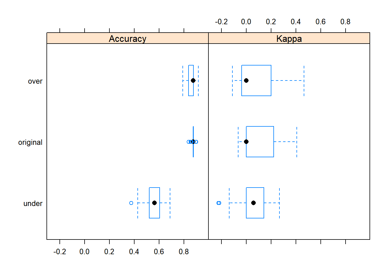
The box and whisker plots below demonstrate the accuracy and kappa for repeated attempts at training each model. For all three, the median kappa values are very low, implying that the models themselves didn’t improve prediction much beyond predicting only the majority class.
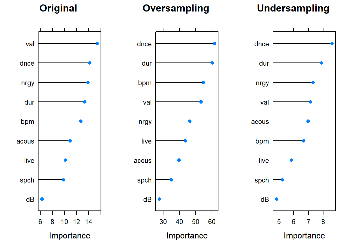
 I found one interesting insight when plotting the variable importance for each model. Variable importance in the Caret package ranges from 0-100. Notice in the plot below, variable importance is much higher in oversampled model than in the undersampled and original models. This suggests that the model did learn some sort of pattern for prediction. However, the predictions from that model didn’t change from those in the original model.
 Based on this brief analysis, it appears that unaccounted for variables such as artist popularity, genre, and possibly the relationship between genre and year, do much of the heavy lifting for a song’s success. And honestly no surprise there. This would explain why artists artists don’t (or do) feel comfortable changing their styles.